A variation of the classification task is semantic segmentation at pixel level. Here, every single pixel in an image is assigned a class. The output is the fully segmented image.

Running It

For a simple scenario it is only necessary to provide the following parameters:

• --dataset-folder specifies the location of the dataset on the machine
• --runner-class semantic_segmentation specifies to use the code for this task and not the standard image classification one

For example:

python RunMe.py --dataset-folder /path/to/dataset --runner-class semantic_segmentation

For the segmentatin task, this structure is slightly different. The data should be split into a train, val, and test set (see prepare your data). Within each of these folders there has to be a sub-folder for the input images and the pixel-wise labelled ground truth, e.g.:

dataset/train/data/
dataset/train/gt/

Each image in the /data folder has a corresponding groun-truth image in the /gt folder. The images that belong together need to have the same name (but they can have a different file extension). The ground truth encoding has to be in the blue channel, with a different number for each class label.

dataset/train/data/page23.png
dataset/train/data/page231.png

dataset/train/gt/page23.png
dataset/train/gt/page231.png

Training and Epoch Definition:

For semantic segmentation at pixel level, the images need to be processes at full resolution. This leads to new challenges for large images, as they requires a lot of memory. To overcome this, the semantic segmentation runner samples random crops from the input image during training and validation. The train / val epoch is as long as the number of crops taken per image multiplied by then number of images in the data subset. During the test phase, the full image in processed with a sliding window with an overlap of 50% (keeping the maximum activation).

Troubleshooting:

See Troubleshooting

Visualize Results

In addition to those provided by the image classification (see perform image classification), the following visualizations are produced:

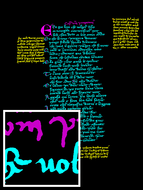
• Visualized segmentation output, where each class is highlighted in a different colour.

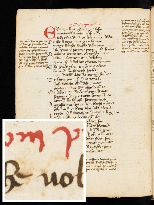
Example input image from the DIVA-HisDB dataset:

Visualization of the pixel-wise labels (here from the ground truth):

Segmentation Output

The output of the segmentation are the pixel-wise labels of the input image. The output image is saved in the same format as the ground truth image. The class labels are encoded in the blue channel of the RGB image.

Customization Options

There are a lot of elements that can be modified in an experiment. Many functionalities are already implemented and accessible through a command line parameters.

See customizing options for a brief overview of the most common ones.

Specifically for the semantic segmentation, there are the following additional options which are important to think about:

• --imgs-in-memory specifies how many images should be loaded into memory at the same time
• --crop-size specifies the size of the crops from the full image used during training and validation
• --crops-per-image specifies how many crops are taken per image during one epoch during training and validation

For a comprehensive list of the possibilities offered by the framework see the latest version of the docs.

Special case: DIVA-HisDB dataset

For the DIVA-HisDB dataset there is a separate runner available, which also provides an output like the DIVA layout analysis evaluator. It also considers the boundary-pixels, which are set to background for the loss computation.