DeepDIVA outputs all of it’s logs to text files that are in the experiment folder, but in addition to that produces visualisations that can be viewed using Tensorboard.

Starting Tensorboard

All visualisations produced by DeepDIVA are logged and viewable using Tensorboard. To view these results, activate an instance of Tensorboard in the following manner.

• Activate the DeepDIVA environment using

source activate deepdiva

• Run the following command to use Tensorboard

tensorboard --logdir /path/to/output-folder --port <port_number>

Tensorboard will then provide a link to view the visualisations in your browser. If you are running DeepDIVA on your local machine, the website can be accessed by going to the link http://localhost:<port_number>

Example

Assume you ran an image classification experiment on your local machine (see Perform Image Classification) and produced logs in the output folder /home/totallynotarobot/my_output/. To activate Tensorboard and view logs, you would:

• Change directory to /home/totallynotarobot/my_output/
• Then run the following command:

tensorboard --logdir ./ --port 6006

Then all the visualisations produced by Tensorboard would be visible on http://localhost:6006.

Note

Usually, it is helpful to have a persistent Tensorboard session running. This can be accomplished using screen or tmux.

Scalars Visualization

In the SCALARS tab of Tensorboard is possible to visualize all the scalar plots produced by DeepDIVA. The standard ones are accuracy (or mAP for the image similarity task) and loss for train, validation and test respectively. Note that test values are not a traditional plot but rather a single point in the chart.

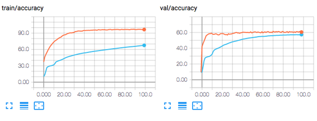
Note that TensorBoard has already a smoothing function integrated which allows you to see the trend of certain distributions more easily. For example, in the next image is visualized the minibatch loss for a model with the smoothing active.

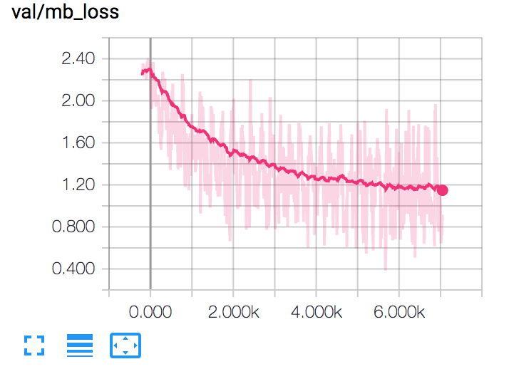
Image Visualization

In the IMAGE tab of Tensorboard is possible to visualize all the images produced by DeepDIVA. Follows a list of them with a brief description.

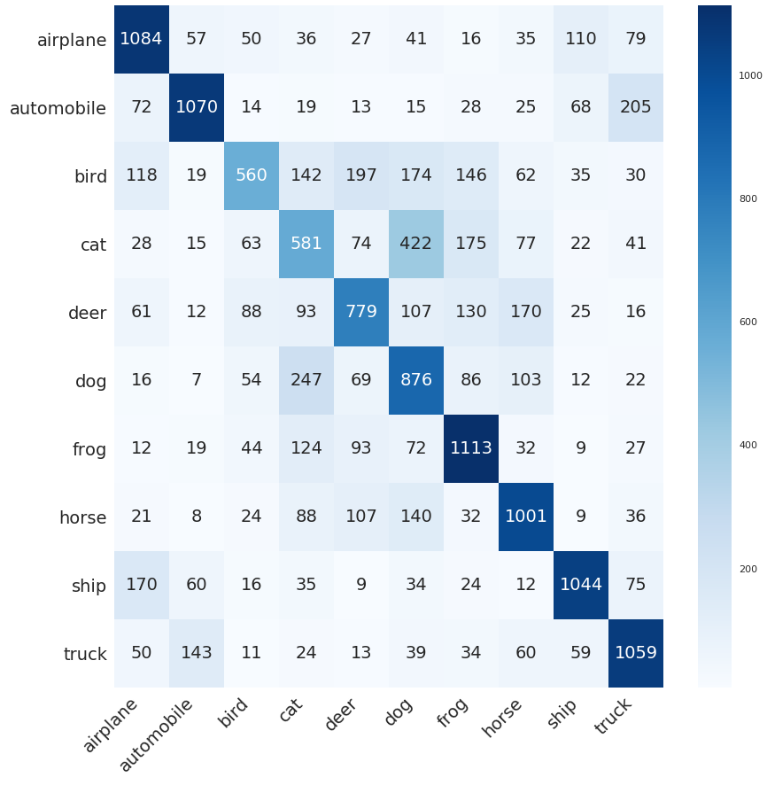
Confusion Matrix

A very common way of asses the performance of a classification system if the confusion matrix. The framework generates one each time the model is validated and tested so that is possible to track the progression of the system over time.

This is an example of one of them evaluated on the CIFAR dataset:

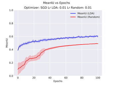
Multiple Runs Aggregations

Drawing conclusions based on a single run is often risky due to the large amount of randomness involved in the process (initialization, order of the training data, …). Therefore the experiments should be run multiple times and the result aggregated. DeepDIVA got that covered and with the parameter --multi-run [int] one can specify to reapeat the same procedure a desired amount of times. The results will then bi available as single runs (as normal) but also in the form of aggregated plots which will make it easier to interpret. In the image below there is an example of a comparison of two systems after multiple runs. The shaded area corresponds to the variance whereas the tick line is the average result.

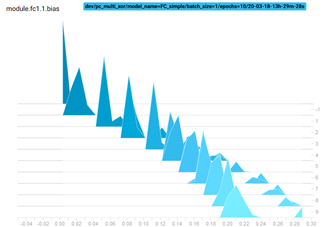
Weights Distribution

The TensorBoard Histogram Dashboard displays how the distribution of some Tensor in your TensorFlow graph has changed over time. It does this by showing many histograms visualizations of your tensor at different points in time.

Here is an example that shows how the bias of a network have evolved during training:

Embeddings

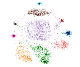
TensorBoard has a built-in visualizer, called the Embedding Projector, for interactive visualization and analysis of high-dimensional data like embeddings. A detailed explanation on how it works and how to use it can be found here.

This is an example of a snapshot of an embedding visualization:

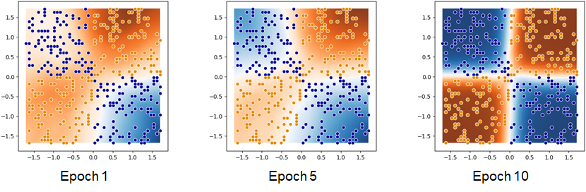
Decision Boundaries

This is a visualization of the decision boundaries of the network. In practice this is realised by asking the model to output a prediction to all points in the grid. The colour of the background represent the output of the model, whereas its intensity the confidence. Strong colour means high confidence, light (more white) colour means low confidence. The points in the foreground represent the samples in the validation set. Their colour reflect the class they belong to.

The following image is an example of a network which learned to solve the continuous XOR problem with three measuring at different epochs:

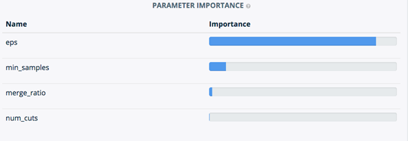
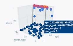
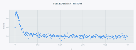
Bayesian Hyper-parameter Optimization With SigOpt

In DeepDIVA we integrated a smarted way to perform hyper-paramter optimization than random or grid search. We use a commercial tool offered by SigOpt which tunes a model’s parameters through state-of-the-art Bayesian optimization.

Here are presented only a very small subset of all useful visualization offered by the tool: